DEM+LBM Examples
Sphere in fluid and the measurement of Stokes Law
This tutorial aims combines most of the concepts introduced in the previous version with the novel coupling between DEM and LBM. The code will introduce a LBM grid where the fluid is accelerated with a constant body force and a sphere is immersed in it. The force over the sphere can be calculated to obtain the drag coefficient.
struct UserData
{
std::ofstream oss_ss;
Vec3_t acc;
double nu;
double R;
Array<Cell *> xmin;
Array<Cell *> xmax;
};
void Setup(LBM::Domain & dom, void * UD)
{
UserData & dat = (*static_cast<UserData *>(UD));
#ifdef USE_OMP
#pragma omp parallel for schedule(static) num_threads(dom.Nproc)
#endif
for (size_t i=0;i<dom.Lat[0].Ncells;i++)
{
Cell * c = dom.Lat[0].Cells[i];
c->BForcef = c->Rho*dat.acc;
}
}
void Report(LBM::Domain & dom, void * UD)
{
UserData & dat = (*static_cast<UserData *>(UD));
if (dom.idx_out==0)
{
String fs;
fs.Printf("%s_force.res",dom.FileKey.CStr());
dat.oss_ss.open(fs.CStr());
dat.oss_ss << Util::_10_6 << "Time" << Util::_8s << "Fx" << Util::_8s << "Fy" << Util::_8s << "Fz" << Util::_8s << "Tx" << Util::_8s << "Ty" << Util::_8s << "Tz" << Util::_8s << "Vx" << Util::_8s << "Fx" << Util::_8s << "F" << Util::_8s << "Rho" << Util::_8s << "Re" << Util::_8s << "CD" << Util::_8s << "CDsphere \n";
}
if (!dom.Finished)
{
double M = 0.0;
double Vx = 0.0;
size_t nc = 0;
Vec3_t Flux = OrthoSys::O;
for (size_t i=0;i<dom.Lat[0].Ncells;i++)
{
Cell * c = dom.Lat[0].Cells[i];
if (c->IsSolid||c->Gamma>1.0e-8) continue;
Vx += (1.0 - c->Gamma)*c->Vel(0);
Flux += c->Rho*c->Vel;
M += c->Rho;
nc++;
}
Vx /=dom.Lat[0].Ncells;
Flux/=M;
M /=nc;
double CD = 2.0*dom.Particles[0]->F(0)/(Flux(0)*Flux(0)/M*M_PI*dat.R*dat.R);
double Re = 2.0*Flux(0)*dat.R/(M*dat.nu);
double CDt = 24.0/Re + 6.0/(1.0+sqrt(Re)) + 0.4;
if (Flux(0)<1.0e-12)
{
Flux = OrthoSys::O;
CD = 0.0;
Re = 0.0;
}
dat.oss_ss << Util::_10_6 << dom.Time << Util::_8s << dom.Particles[0]->F(0) << Util::_8s << dom.Particles[0]->F(1) << Util::_8s << dom.Particles[0]->F(2) << Util::_8s << dom.Particles[0]->T(0) << Util::_8s << dom.Particles[0]->T(1) << Util::_8s << dom.Particles[0]->T(2) << Util::_8s << Vx << Util::_8s << Flux(0) << Util::_8s << norm(Flux) << Util::_8s << M << Util::_8s << Re << Util::_8s << CD << Util::_8s << CDt << std::endl;
}
else
{
dat.oss_ss.close();
}
}
int main(int argc, char **argv) try
{
if (argc<2) throw new Fatal("This program must be called with one argument: the name of the data input file without the '.inp' suffix.\nExample:\t %s filekey\n",argv[0]);
size_t Nproc = 1;
if (argc==3) Nproc=atoi(argv[2]);
String filekey (argv[1]);
String filename (filekey+".inp");
if (!Util::FileExists(filename)) throw new Fatal("File <%s> not found",filename.CStr());
ifstream infile(filename.CStr());
String ptype;
bool Render = true;
size_t nx = 100;
size_t ny = 50;
size_t nz = 50;
double nu = 0.01;
double dx = 1.0;
double dt = 1.0;
double Dp = 0.1;
double R = 10.0;
double w = 0.001;
double ang= 0.0;
double Tf = 40000.0;
{
infile >> ptype; infile.ignore(200,'\n');
infile >> Render; infile.ignore(200,'\n');
infile >> nx; infile.ignore(200,'\n');
infile >> ny; infile.ignore(200,'\n');
infile >> nz; infile.ignore(200,'\n');
infile >> nu; infile.ignore(200,'\n');
infile >> dx; infile.ignore(200,'\n');
infile >> dt; infile.ignore(200,'\n');
infile >> Dp; infile.ignore(200,'\n');
infile >> R; infile.ignore(200,'\n');
infile >> w; infile.ignore(200,'\n');
infile >> ang; infile.ignore(200,'\n');
infile >> Tf; infile.ignore(200,'\n');
}
LBM::Domain Dom(D3Q15, nu, iVec3_t(nx,ny,nz), dx, dt);
Dom.Step = 1;
Dom.Sc = 0.0;
UserData dat;
Dom.UserData = &dat;
dat.acc = Vec3_t(Dp,0.0,0.0);
dat.R = R;
dat.nu = nu;
for (int i=0;i<nx;i++)
for (int j=0;j<ny;j++)
for (int k=0;k<nz;k++)
{
Vec3_t v0(0.0,0.0,0.0);
Dom.Lat[0].GetCell(iVec3_t(i,j,k))->Initialize(1.0,v0);
}
if (ptype=="sphere") Dom.AddSphere(-1,Vec3_t(0.5*nx*dx,0.5*ny*dx,0.5*nz*dx),R,3.0);
else if (ptype=="tetra" )
{
double e = pow(sqrt(2)*M_PI,1.0/3.0)*2*R;
Dom.AddTetra(-1,Vec3_t(0.5*nx*dx,0.5*ny*dx,0.5*nz*dx),0.05*e,e,3.0,M_PI/4.0,&OrthoSys::e2);
Quaternion_t q;
NormalizeRotation(35.26*M_PI/180.0,OrthoSys::e1,q);
Dom.Particles[0]->Rotate(q,Dom.Particles[0]->x);
NormalizeRotation(ang*M_PI/180.0,OrthoSys::e2,q);
Dom.Particles[0]->Rotate(q,Dom.Particles[0]->x);
}
else if (ptype=="cube" )
{
double e = pow(M_PI/6.0,1.0/3.0)*2*R;
Dom.AddCube(-1,Vec3_t(0.5*nx*dx,0.5*ny*dx,0.5*nz*dx),0.05*e,e,3.0,ang*M_PI/180.0,&OrthoSys::e2);
}
else
{
DEM::Particle * Pa = new DEM::Particle(-1, ptype.CStr(), 0.05*R, 3.0, R );
Dom.Particles.Push(Pa);
Vec3_t t(0.5*nx,0.5*ny,0.5*nz);
Pa->Position(t);
}
Dom.Particles[0]->FixVeloc();
Dom.Particles[0]->w = Vec3_t(0.0,0.0,w);
//Solving
Dom.Solve(Tf,0.01*Tf,Setup,Report,filekey.CStr(),Render,Nproc);
}
MECHSYS_CATCH
UserData Structure
The first step is to define the UserData structure as in the case of the flow past a cylinder
                                struct UserData
                                {
                                    std::ofstream      oss_ss;
                                    Vec3_t                acc;
                                    double                 nu;
                                    double                  R;
                                };
The first variable is an object of the class std::ofstream which is a class
from C++ for output files. The vector acc will contain the acceleration which
is chosen by the user. Part of the output is to report the Reynolds number which requires both the equivalent radius
of the particle R and the viscosity of the fluid nu.
Setup Function
As in the example of flow around cylinder a user defined function is used to internally modified some variables within the time for loop. In this case the function will only applied the body force for each LBM cell providing a constant acceleration.
                                void Setup(LBM::Domain & dom, void * UD)
                                {
                                    UserData & dat = (*static_cast<UserData *>(UD));
                                #ifdef USE_OMP
                                    #pragma omp parallel for schedule(static) num_threads(dom.Nproc)
                                #endif
                                    for (size_t i=0;i<dom.Lat[0].Ncells;i++)
                                    {
                                        Cell * c   = dom.Lat[0].Cells[i];
                                        c->BForcef = c->Rho*dat.acc;
                                    }
                                }
As can be seen, the for loop modifies the variable BForcef of the Cell class by assigning it a value of the cell density (c->Rho) times the imposed acceleration dat.acc. The #pragma preamble is used for parallelization of
this for loop.
Report Function
Since the goal of this test is to measure the drag coefficient, it is important to report the force over the particle for each time step. The Report function help us to achieve this goal.
                                void Report(LBM::Domain & dom, void * UD)
                                {
                                    UserData & dat = (*static_cast<UserData *>(UD));
                                    if (dom.idx_out==0)
                                    {
                                        String fs;
                                        fs.Printf("%s_force.res",dom.FileKey.CStr());
                                        dat.oss_ss.open(fs.CStr());
                                        dat.oss_ss << Util::_10_6 << "Time" << Util::_8s << "Fx" << Util::_8s << "Fy" << Util::_8s << "Fz" << Util::_8s << "Tx" << Util::_8s << "Ty" << Util::_8s << "Tz" << Util::_8s << "Vx" << Util::_8s << "Fx" << Util::_8s << "F" << Util::_8s << "Rho" << Util::_8s << "Re" << Util::_8s << "CD" << Util::_8s << "CDsphere \n";
                                    }
                                    if (!dom.Finished)
                                    {
                                        double M    = 0.0;
                                        double Vx   = 0.0;
                                        size_t nc   = 0;
                                        Vec3_t Flux = OrthoSys::O;
                                        for (size_t i=0;i<dom.Lat[0].Ncells;i++)
                                        {
                                            Cell * c = dom.Lat[0].Cells[i];
                                            if (c->IsSolid||c->Gamma>1.0e-8) continue;
                                            Vx   += (1.0 - c->Gamma)*c->Vel(0);
                                            Flux += c->Rho*c->Vel;
                                            M    += c->Rho;
                                            nc++;
                                        }
                                        Vx  /=dom.Lat[0].Ncells;
                                        Flux/=M;
                                        M   /=nc;
                                        double CD  = 2.0*dom.Particles[0]->F(0)/(Flux(0)*Flux(0)/M*M_PI*dat.R*dat.R);
                                        double Re  = 2.0*Flux(0)*dat.R/(M*dat.nu);
                                        double CDt = 24.0/Re + 6.0/(1.0+sqrt(Re)) + 0.4;
                                        if (Flux(0)<1.0e-12)
                                        {
                                            Flux = OrthoSys::O;
                                            CD = 0.0;
                                            Re = 0.0;
                                        }

                                        dat.oss_ss << Util::_10_6 << dom.Time << Util::_8s << dom.Particles[0]->F(0) << Util::_8s << dom.Particles[0]->F(1) << Util::_8s << dom.Particles[0]->F(2) << Util::_8s << dom.Particles[0]->T(0) << Util::_8s << dom.Particles[0]->T(1) << Util::_8s << dom.Particles[0]->T(2) << Util::_8s << Vx << Util::_8s << Flux(0) << Util::_8s << norm(Flux) << Util::_8s << M << Util::_8s << Re << Util::_8s << CD << Util::_8s << CDt << std::endl;
                                    }
                                    else
                                    {
                                        dat.oss_ss.close();
                                    }
                                }
The first exception (dom.idx_out==0) checks if the simulation is running
the first instance of the time for loop. It will open the file "%s_force.res" (where %s will be replace by the filekey
introduced in the function Solve). Once opened, the function will write a
header on the file with the tags for the columns storing the time, the components of the force over the particle (F)
, the torque (T), the Reynolds number (Re) and the drag coefficient (CD).
The second exception (!dom.Finished) checks if the last instance of the
time for loop has not been reached (i.e. that if the simulation is still running). The it will go through each cell to
calculate the average velocity. With this, the drag coefficient and the Reynolds number are calculated and stored in
the output file. In particular, the drag coefficient requires to force over the particle which is obtained from the
variable dom.Particles[0]->F. Finally once the last instance of the time for loop is reached, the output file is closed and flushed
out.
The main loop
As in the previous examples, the main loop is used to set the scene for the simulation and call the Solve function. One difference between the previous examples is that now an
input file must be provided which allows to make changes on the parameters without having to recompile to code again.
the input file (test_input.inp) includes all the key variables for the study
                                sphere    = ptype     Particle type
                                0         = Render    Produce visualization files?
                                240       = nx        x dimension of lbm grid
                                60        = ny        y dimension of lbm grid
                                60        = nz        z dimension of lbm grid
                                1.0       = nu        viscosity of the fluid
                                0.4       = dx        grid size
                                1.6e-2    = dt        time step
                                3.1e-2    = Dp        fluid acceleration
                                3.6       = R         particle size
                                0.00      = w         angular velocity
                                45.0      = ang        angle of the body around the z axis
                                1.0e3     = Tf        time
Each of this variables are read within the main loop in the following section
                                infile >> ptype;        infile.ignore(200,'\n');
                                infile >> Render;       infile.ignore(200,'\n');
                                infile >> nx;           infile.ignore(200,'\n');
                                infile >> ny;           infile.ignore(200,'\n');
                                infile >> nz;           infile.ignore(200,'\n');
                                infile >> nu;           infile.ignore(200,'\n');
                                infile >> dx;           infile.ignore(200,'\n');
                                infile >> dt;           infile.ignore(200,'\n');
                                infile >> Dp;           infile.ignore(200,'\n');
                                infile >> R;            infile.ignore(200,'\n');
                                infile >> w;            infile.ignore(200,'\n');
                                infile >> ang;          infile.ignore(200,'\n');
                                infile >> Tf;           infile.ignore(200,'\n');
And as such, the input values become variables of the main loop that can be used to define the problem parameters.
For instance, one key variable is the string ptype which determines the
particle type and has four possible options (sphere, tetra, cube and the name of a JSON file to import a mesh
particle). Once the particle is defined, it is added to the domain. For example, for the case of a sphere we have
if (ptype=="sphere") Dom.AddSphere(-1,Vec3_t(0.5*nx*dx,0.5*ny*dx,0.5*nz*dx),R,3.0);
Adds a sphere at the center of the domain with radius given by the variable R and density equal to 3.0. Most of the functions to add particles come from the DEM domain and the
spheropolyhedra method is embedded into the LBM domain as well so that complex shapes particles can interact with each
other and with the fluid.
The last line before the Solve function fix to zero the velocity of the particle
by means of the function FixVeloc and assign an angular velocity along the z
axis. When the particle has its velocities fixed, neither the forces or torques will change the velocity or angular
velocity although they can still be recorded. That ensures that the particle will remain at the center and will keep
spinning.
                                    Dom.Particles[0]->FixVeloc();
                                    Dom.Particles[0]->w = Vec3_t(0.0,0.0,w);
Results
To run the simulation the command ./test_spherefluid test_input 8 must be
entered where 8 can be replaced for any other number of cores. This example is particularly time consumming so it is
advised to use all the available cores. By plotting the results of the file test_input_force.res, a comparison can be
done with empirical formulae found from
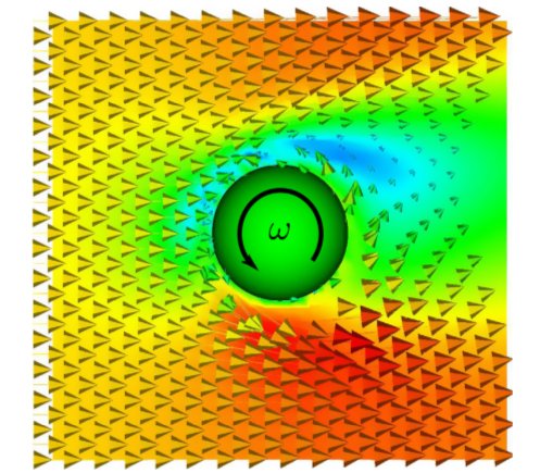
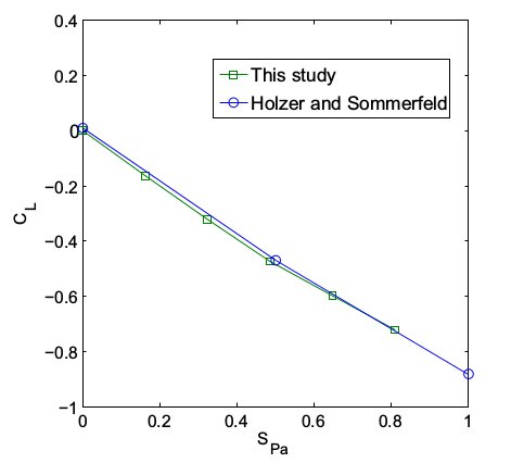
experiments for the drag coefficient of a sphere. In the next images, the fluid velocity field and the results for the
lift coefficient for several angular velocities are presented by comparison. The results are taken from this
paper which was written while Mechsys was developed. Please
refer to it for further details.